Simulation Studies

Mixed Effects Models

R Packages

library(tidyverse)
library(mvtnorm)
library(brms)
theme_set(theme_bw())

Longitudinal Studies

Longitudinal Studies
Linear Mixed-Effects Models
Generalized Linear Mixed-Effects Models
Multilevel Models

Longitudinal Studies

Longitudinal studies are designed to determine whether there are time effects on an outcome of interest.

The data typically recorded on an experimental unit multiple times.

The repeated measurements are considered correlated due to sharing the experimental unit.

Correlated Outcomes

Correlated outcomes causes the standard error of the estimated to be inflated.

Therefore, inferential procedures are unreliable.

Data Structure

\[ Y_{i} = (Y_{i1}, Y_{i2}, \ldots, Y_{in_i}) \]

Modelling

Generalized Least Squares
Generalized Estimating Equations
Mixed Effects Models

Linear Mixed-Effects Models

Longitudinal Studies
Linear Mixed-Effects Models
Generalized Linear Mixed-Effects Models
Multilevel Models

Linear Models

\[ Y_{ij} = \beta_0 + \beta_1X_{ij} + \varepsilon_{ij} \]

Random Effects Model

\[ Y_{ij} = b_{0i} + b_{1i}X_{ij} + \varepsilon_i \]

Mixed Effects Model

\[ Y_{ij} = \beta_0 + \beta_1X_{ij} + b_{0i} + b_{1i}X_{ij} + \varepsilon_{ij} \]

\(b_{i0}\sim N(0, \sigma^2_{b0})\)
\(b_{i1}\sim N(0, \sigma^2_{b1})\)
\(\varepsilon_{ij} \sim N(0, \sigma^2_\varepsilon)\)
\(b_i \perp \varepsilon_{ij}\)

Simulation Study

500 Units (patients)
For each unit, 5 repeated measurements
\(Y_{ij} = 4 + 1.9 X_{i1} + 2.3 t_j + b_{i0} + b_{i1} t_j + \varepsilon_{ij}\)
\(\varepsilon_{ij}\sim N(0, 1.1^2)\)
\(b_{i0}\sim N(0, 1.8^2)\)
\(b_{i1}\sim N(0,1.5^2)\)

Simulation

Code

df <- tibble()
beta0 <- 4
beta1 <- 1.9
beta2 <- 2.3
t <- 0:4

n <- 500
for(i in 1:n){
  b0 <- rnorm(1, sd = 1.8)
  b1 <- rnorm(1, sd = 1.5)
  x.vec <- rmvnorm(1, sigma = diag(rep(1, 5))) |> as.vector()
  y <- beta0 + beta1 * t + beta2 * x.vec + b0 + b1 * t  + rnorm(5, sd = 1.1) |> as.vector()
  df <- bind_rows(df,
                  tibble(y = y, x = x.vec, t = t, id = i))

}

Bayesian Analysis in R

Code

brm(y ~ x + t + (t|id),
    data = df,
    family = gaussian(),
    cores = 4)

Generalized Linear Mixed-Effects Models

Longitudinal Studies
Linear Mixed-Effects Models
Generalized Linear Mixed-Effects Models
Multilevel Models

GLMM

\[ g\{E(Y_{ij})\} = \beta_0 + \beta_1X_{ij} + b_{0i} + b_{1i}X_{ij} \]

Simulation Study

500 Units (patients)
For each unit, 5 repeated measurements
\(g\{E(Y_{ij})\} = 2 - 1.56 X_{i1} - 1.3 t_j + b_{i0} + b_{i1} t_j\)
\(Y_{ij} \sim Bern(p_{ij})\)
\(b_{i0}\sim N(0, 1.8^2)\)
\(b_{i1}\sim N(0,1.5^2)\)

Simulation

Code

df <- tibble()
beta0 <- 2
beta1 <- -1.56
beta2 <- -1.3
t <- 0:4

n <- 500
for(i in 1:n){
  b0 <- rnorm(1, sd = 1.8)
  b1 <- rnorm(1, sd = 1.5)
  x.vec <- rmvnorm(1, sigma = diag(rep(1, 5))) |> as.vector()
  mu <- boot::inv.logit(beta0 + beta1 * t + beta2 * x.vec + b0 + b1 * t)
  y <- rbinom(5, 1, mu)
  df <- bind_rows(df,
                  tibble(y = y, x = x.vec, t = t, id = i))

}

Bayesian Analysis in R

Code

brm(y ~ t + x + (t|id),
    data = df,
    family = bernoulli(),
    cores = 4)

Multilevel Models

Longitudinal Studies
Linear Mixed-Effects Models
Generalized Linear Mixed-Effects Models
Multilevel Models

Multilevel Models

Multilevel models are utilized to account for correlation among multiple grouping settings.

Longitudinal Biomedical Study

Multilevel Models can be used to model patients in a facility, and repeated measurements in a patient.

The first level is the facility. There are a set number of facilities in a study.

The next level are the patients within a facility. Additionally, each patient has a set of observations.

It is thought that the patients within the facility share a number of characteristics. This will bias the standard errors in a model if not accounted for.

Data Structure

\(Y_i=(Y_{i1}, Y_{i2}, \ldots, Y_{in_{i}}) ^\mathrm T\): A vector containing all the outcomes in a facility.
\(Y_{ij}=(Y_{ij1}, Y_{ij2}, \ldots, Y_{ijn_{ij}}) ^\mathrm T\) A vector containing all the the outcomes in a patient.
\(Y_{ijk}\): An individual outcome.

Model

\[ Y_{ijk} = \beta_0 + \beta_1 X_{ij} + \beta_2 t_{ijk} + b_i + b_{ij} + \varepsilon_{ijk} \]

Simulation Study

500 Facilities
For each facility, there are 30 patients
For each patient there are 5 repeated measurements
\(Y_{ijk} = 2 - 1.56 X_{i1} - 1.3 t_j + b_{ij} + b_{i} + \varepsilon_{ijk}\)
\(\varepsilon_{ijk} \sim N(0, 4)\)
\(b_{i}\sim N(0, .6^2)\)
\(b_{ij}\sim N(0,1.1^2)\)

Simulation

Code

df <- tibble()
beta0 <- 2
beta1 <- -1.56
beta2 <- -1.3
t <- 0:4

n <- 25
nn <- 30
j <- 1

for(i in 1:n){
  xi <- rnorm(1, sd = .6)
  for(ii in 1:nn){
    b0 <- rnorm(1, sd = 1.1)
    x.vec <- rmvnorm(1, sigma = diag(rep(1, 5))) |> as.vector()
    y <- beta0 + beta1 * t + beta2 * x.vec + 
                            b0 + xi + rnorm(5, sd = 2) |> 
      as.vector()
    df <- bind_rows(df,
                    tibble(y = y, x = x.vec, t = t, 
                           id = i, id2 = ii, jid = j))
    j <- j + 1
  }
}

Bayesian Analysis in R

Code

brm(y ~ x + t + (1|jid) + (1|id),
    data = df,
    family = gaussian(),
    iter = 2000,
    cores = 4)

Frog Study

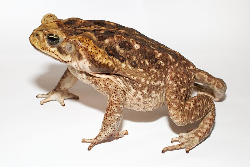
Frog Species

Two of the frog species seems similar to each other.

Could they be evolutionarily related to each other?

We need to account the relatedness using random effects.

Random Effects on Species

\[ \left(\begin{array}{c}S_1\\S_2\\S_3\end{array}\right) \sim N\left\{\left(\begin{array}{c}0\\0\\0\end{array}\right), \left(\begin{array}{ccc}\sigma_{1}^2 & \sigma_{12} & \sigma_{13}\\\sigma_{12} & \sigma_{2}^2 & \sigma_{23}\\\sigma_{13} & \sigma_{23} & \sigma_{3}^2\end{array}\right) \right\} \]

Model

\[ Y_{ijk} = \beta_0 + \beta_1 X_{i1} + \beta_2 t_j + b_{ij} + b_{i} + b_{sp(ij)} + \varepsilon_{ijk} \]

Simulation Study

15 Housing Unit
For each Housing Unit, there are 15 frogs
For each Housing Unit, there are 5 frogs of each species
For each frog, there are 4 repeated measurements
\(Y_{ijk} = 2 - 1.56 X_{i1} - 1.3 t_j + b_{ij} + b_{i} + b_{sp(ij)} + \varepsilon_{ijk}\)
\(\varepsilon_{ijk} \sim N(0, 4)\)
\(b_{i}\sim N(0, .6^2)\)
\(b_{ij}\sim N(0,1.1^2)\)
\(b_{sp(ij)} \sim N_3(0, \Sigma)\)

Simulation

Code

x1 <- c(1, 0.80, 0.10)
x2 <- c(0.80, 1, 0.43)
x3 <- c(0.10, 0.43, 1)
corr_x <- as.matrix(rbind(x1, x2, x3))
cov_x <- 2.2^2 * corr_x 
spe_id <- rep(1:3, times = 10)
spe_re <- rmvnorm(1, sigma = cov_x)

rownames(corr_x) <- c("A", "B", "C")
colnames(corr_x) <- c("A", "B", "C")

df <- tibble()
beta0 <- 2
beta1 <- -1.56
beta2 <- -1.3
t <- 0:3

n <- 15
nn <- 30
j <- 1

for(i in 1:n){
  xi <- rnorm(1, sd = .6)
  for(ii in 1:nn){
    b0 <- rnorm(1, sd = 1.1)
    x.vec <- rmvnorm(1, sigma = diag(rep(1, 4))) |> as.vector()
    y <- beta0 + beta1 * t + beta2 * x.vec + 
          b0 + xi + spe_re[spe_id[ii]] + rnorm(4, sd = 2) |> 
      as.vector()
    df <- bind_rows(df,
                    tibble(y = y, x = x.vec, t = t, 
                           id = i, id2 = ii, jid = j, 
                           spe = case_when(spe_id[ii] == 1 ~ "A",
                                           spe_id[ii] == 2 ~ "B",
                                           spe_id[ii] == 3 ~ "C")))
    j <- j + 1
  }
}

Bayesian Analysis in R

Code

brm(y ~ x + t + (1|jid) + (1|id) + (1|gr(spe, cov = A)),
    data = df,
    data2 = list(A = corr_x),
    family = gaussian(),
    prior = c(
      prior(normal(0, 10), "b"),
      prior(normal(0, 50), "Intercept"),
      prior(student_t(3, 0, 20), "sd"),
      prior(student_t(3, 0, 20), "sigma")
    ),
    control = list(adapt_delta = 0.99,
                   max_treedepth = 30),
    iter = 4000,
    cores = 4)