Monte Carlo Methods
Random Variable Generation
Flipping a Coin
| Outcome | Head | Tails |
| Probability | 0.5 | 0.5 |

Rolling a Die
| Outcome | 1 | 2 | 3 | 4 | 5 | 6 |
| Probability | 1/6 | 1/6 | 1/6 | 1/6 | 1/6 | 1/6 |

Rolling a Die

Bernoulli Distribution (n = 1, p = 0.1; Biased Coin Flip)
Code
p <- 0.1
x <- rbinom(50000, 1, p)
p1 <- x |> tibble() |>
ggplot(aes(x)) +
geom_bar(aes(y = (..count..)/sum(..count..))) +
ylab("Probability") +
ggtitle("PMF") +
theme_bw()
p2 <- 0:1 |> pbinom(1, p) |> tibble(x = 0:1, y = _) |>
ggplot(aes(x,y)) +
geom_step() +
theme_bw() +
ggtitle("CDF") +
ylab(paste0("P(X","\u2264"," x)"))
p1 + p2
Distribution (n = 30, p = 0.1)
Code
p <- 0.1
x <- rbinom(50000, 30, p)
p1 <- x |> tibble() |>
ggplot(aes(x)) +
geom_bar(aes(y = (..count..)/sum(..count..))) +
xlim(c(0,30)) +
ylab("Probability") +
ggtitle("PMF") +
theme_bw()
p2 <- 0:30 |> pbinom(30, p) |> tibble(x = 0:30, y = _) |>
ggplot(aes(x,y)) +
geom_step() +
theme_bw() +
ggtitle("CDF") +
ylab(paste0("P(X","\u2264"," x)"))
p1 + p2
Distribution (n = 30, p = 0.5)
Code
p <- 0.5
x <- rbinom(50000, 30, p)
p1 <- x |> tibble() |>
ggplot(aes(x)) +
geom_bar(aes(y = (..count..)/sum(..count..))) +
xlim(c(0,30)) +
ylab("Probability") +
ggtitle("PMF") +
theme_bw()
p2 <- 0:30 |> pbinom(30, p) |> tibble(x = 0:30, y = _) |>
ggplot(aes(x,y)) +
geom_step() +
theme_bw() +
ggtitle("CDF") +
ylab(paste0("P(X","\u2264"," x)"))
p1 + p2
Distribution (n = 30, p = 0.85)
Code
p <- 0.85
x <- rbinom(50000, 30, p)
p1 <- x |> tibble() |>
ggplot(aes(x)) +
geom_bar(aes(y = (..count..)/sum(..count..))) +
xlim(c(0,30)) +
ylab("Probability") +
ggtitle("PMF") +
theme_bw()
p2 <- 0:30 |> pbinom(30, p) |> tibble(x = 0:30, y = _) |>
ggplot(aes(x,y)) +
geom_step() +
theme_bw() +
ggtitle("CDF") +
ylab(paste0("P(X","\u2264"," x)"))
p1 + p2
Distribution (\(\lambda\) = 3.5)
Code
p <- 3.5
x <- rpois(50000, p)
p1 <- x |> tibble() |>
ggplot(aes(x)) +
geom_bar(aes(y = (..count..)/sum(..count..))) +
ylab("Probability") +
ggtitle("PMF") +
theme_bw()
p2 <- 0:max(x) |> ppois(p) |> tibble(x = 0:max(x), y = _) |>
ggplot(aes(x,y)) +
geom_step() +
theme_bw() +
ggtitle("CDF") +
ylab(paste0("P(X","\u2264"," x)"))
p1 + p2
Distribution (\(\lambda\) = 34.5)
Code
p <- 34.5
x <- rpois(50000, p)
p1 <- x |> tibble() |>
ggplot(aes(x)) +
geom_bar(aes(y = (..count..)/sum(..count..))) +
ylab("Probability") +
ggtitle("PMF") +
theme_bw()
p2 <- 0:max(x) |> ppois(p) |> tibble(x = 0:max(x), y = _) |>
ggplot(aes(x,y)) +
geom_step() +
theme_bw() +
ggtitle("CDF") +
ylab(paste0("P(X","\u2264"," x)"))
p1 + p2
Distribution (r = 11, p = 0.1)
Code
p <- 0.1
x <- rnbinom(50000,11, p)
p1 <- x |> tibble() |>
ggplot(aes(x)) +
geom_bar(aes(y = (..count..)/sum(..count..))) +
ylab("Probability") +
ggtitle("PMF") +
theme_bw()
p2 <- 0:max(x) |> pnbinom(11, p) |> tibble(x = 0:max(x), y = _) |>
ggplot(aes(x,y)) +
geom_step() +
theme_bw() +
ggtitle("CDF") +
ylab(paste0("P(X","\u2264"," x)"))
p1 + p2
Distribution (r = 11, p = 0.45)
Code
p <- 0.45
x <- rnbinom(50000, 11, p)
p1 <- x |> tibble() |>
ggplot(aes(x)) +
geom_bar(aes(y = (..count..)/sum(..count..))) +
ylab("Probability") +
ggtitle("PMF") +
theme_bw()
p2 <- 0:max(x) |> pnbinom(11, p) |> tibble(x = 0:max(x), y = _) |>
ggplot(aes(x,y)) +
geom_step() +
theme_bw() +
ggtitle("CDF") +
ylab(paste0("P(X","\u2264"," x)"))
p1 + p2
Distribution (r = 11, p = 0.63)
Code
p <- 0.63
x <- rnbinom(50000, 11, p)
p1 <- x |> tibble() |>
ggplot(aes(x)) +
geom_bar(aes(y = (..count..)/sum(..count..))) +
ylab("Probability") +
ggtitle("PMF") +
theme_bw()
p2 <- 0:max(x) |> pnbinom(11, p) |> tibble(x = 0:max(x), y = _) |>
ggplot(aes(x,y)) +
geom_step() +
theme_bw() +
ggtitle("CDF") +
ylab(paste0("P(X","\u2264"," x)"))
p1 + p2
Distribution (a = 4, b = 25)
Code
a <- 4
b <- 25
x <- seq(a, b, length.out = 1000)
p1 <- dunif(x, a, b) |> tibble(x = x, y = _) |>
ggplot(aes(x, y)) +
geom_line() +
ylab("Density") +
ggtitle("PDF") +
theme_bw()
p2 <- punif(x, a, b) |> tibble(x = x, y = _) |>
ggplot(aes(x,y)) +
geom_line() +
theme_bw() +
ggtitle("CDF") +
ylab(paste0("P(X","\u2264"," x)"))
p1 + p2
Distribution (a = 0, b = 1)
Code
a <- 0
b <- 1
x <- seq(a, b, length.out = 1000)
p1 <- dunif(x, a, b) |> tibble(x = x, y = _) |>
ggplot(aes(x, y)) +
geom_line() +
ylab("Density") +
ggtitle("PDF") +
theme_bw()
p2 <- punif(x, a, b) |> tibble(x = x, y = _) |>
ggplot(aes(x,y)) +
geom_line() +
theme_bw() +
ggtitle("CDF") +
ylab(paste0("P(X","\u2264"," x)"))
p1 + p2
Distribution (\(\mu\) = 34, \(\sigma^2\) = 5)
Code
a <- 25
b <- 45
x <- seq(a, b, length.out = 1000)
p1 <- dnorm(x, 34, sqrt(5)) |> tibble(x = x, y = _) |>
ggplot(aes(x, y)) +
geom_line() +
ylab("Density") +
ggtitle("PDF") +
theme_bw()
p2 <- pnorm(x, 34, sqrt(5)) |> tibble(x = x, y = _) |>
ggplot(aes(x,y)) +
geom_line() +
theme_bw() +
ggtitle("CDF") +
ylab(paste0("P(X","\u2264"," x)"))
p1 + p2
Distribution (\(\mu\) = -8, \(\sigma^2\) = 10)
Code
a <- -20
b <- 4
x <- seq(a, b, length.out = 1000)
p1 <- dnorm(x, -8, sqrt(10)) |> tibble(x = x, y = _) |>
ggplot(aes(x, y)) +
geom_line() +
ylab("Density") +
ggtitle("PDF") +
theme_bw()
p2 <- pnorm(x, -8, sqrt(10)) |> tibble(x = x, y = _) |>
ggplot(aes(x,y)) +
geom_line() +
theme_bw() +
ggtitle("CDF") +
ylab(paste0("P(X","\u2264"," x)"))
p1 + p2
Distribution (\(\alpha\) = 1.5, \(\beta\) = 2.6)
Code
y <- rgamma(1000, 1.5, 2.6)
a <- 0
b <- 10
x <- seq(a, b, length.out = 1000)
p1 <- dgamma(x, 1.5, 2.6) |> tibble(x = x, y = _) |>
ggplot(aes(x, y)) +
geom_line() +
ylab("Density") +
ggtitle("PDF") +
theme_bw()
p2 <- pgamma(x, 1.5, 2.6) |> tibble(x = x, y = _) |>
ggplot(aes(x,y)) +
geom_line() +
theme_bw() +
ggtitle("CDF") +
ylab(paste0("P(X","\u2264"," x)"))
p1 + p2
Distribution (\(\alpha\) = 3.5, \(\beta\) = 1.6)
Code
y <- rgamma(1000, 3.5, 1.6)
a <- 0
b <- 10
x <- seq(a, b, length.out = 1000)
p1 <- dgamma(x, 3.5, 1.6) |> tibble(x = x, y = _) |>
ggplot(aes(x, y)) +
geom_line() +
ylab("Density") +
ggtitle("PDF") +
theme_bw()
p2 <- pgamma(x, 3.5, 1.6) |> tibble(x = x, y = _) |>
ggplot(aes(x,y)) +
geom_line() +
theme_bw() +
ggtitle("CDF") +
ylab(paste0("P(X","\u2264"," x)"))
p1 + p2
Distribution (\(\alpha\) = 5.2, \(\beta\) = 1.6)
Code
y <- rgamma(1000, 5.2, 1.6)
a <- 0
b <- 10
x <- seq(a, b, length.out = 1000)
p1 <- dgamma(x, 5.2, 1.6) |> tibble(x = x, y = _) |>
ggplot(aes(x, y)) +
geom_line() +
ylab("Density") +
ggtitle("PDF") +
theme_bw()
p2 <- pgamma(x, 5.2, 1.6) |> tibble(x = x, y = _) |>
ggplot(aes(x,y)) +
geom_line() +
theme_bw() +
ggtitle("CDF") +
ylab(paste0("P(X","\u2264"," x)"))
p1 + p2
Distribution (\(\alpha\) = 5.2, \(\beta\) = 1.6)
Code
y <- rbeta(1000, 5.2, 1.6)
a <- 0
b <- 1
x <- seq(a, b, length.out = 1000)
p1 <- dbeta(x, 5.2, 1.6) |> tibble(x = x, y = _) |>
ggplot(aes(x, y)) +
geom_line() +
ylab("Density") +
ggtitle("PDF") +
theme_bw()
p2 <- pbeta(x, 5.2, 1.6) |> tibble(x = x, y = _) |>
ggplot(aes(x,y)) +
geom_line() +
theme_bw() +
ggtitle("CDF") +
ylab(paste0("P(X","\u2264"," x)"))
p1 + p2
Distribution (\(\alpha\) = 1.3, \(\beta\) = 1.6)
Code
y <- rbeta(1000, 1.3, 1.6)
a <- 0
b <- 1
x <- seq(a, b, length.out = 1000)
p1 <- dbeta(x, 1.3, 1.6) |> tibble(x = x, y = _) |>
ggplot(aes(x, y)) +
geom_line() +
ylab("Density") +
ggtitle("PDF") +
theme_bw()
p2 <- pbeta(x, 1.3, 1.6) |> tibble(x = x, y = _) |>
ggplot(aes(x,y)) +
geom_line() +
theme_bw() +
ggtitle("CDF") +
ylab(paste0("P(X","\u2264"," x)"))
p1 + p2
Distribution (\(\alpha\) = .72, \(\beta\) = .76)
Code
a <- .72
b <- .76
x <- seq(0, 1, length.out = 1000)
p1 <- dbeta(x, a, b) |> tibble(x = x, y = _) |>
ggplot(aes(x, y)) +
geom_line() +
ylab("Density") +
ggtitle("PDF") +
theme_bw()
p2 <- pbeta(x, a, b) |> tibble(x = x, y = _) |>
ggplot(aes(x,y)) +
geom_line() +
theme_bw() +
ggtitle("CDF") +
ylab(paste0("P(X","\u2264"," x)"))
p1 + p2
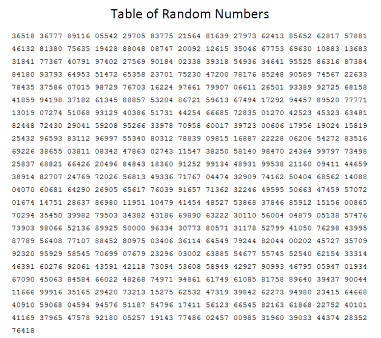
Generating Random Numbers

Generating Random Numbers

Generating Random Numbers
Generating Random Numbers
Inverse-Transform Method

Simulating an Exponential RV
\[ X \sim Exp(2) \]

Simulating an Exponential RV

Poisson Distribution

Poisson Distribution
Code
finder <- function(u){
  x <- 0
  condition <- TRUE
  while (condition) {
    uu <- ppois(x, lambda = 6)
    condition <- uu <= u
    if(condition){
      x <- x + 1
    }
  }
  return(x)
}
xx <- sapply(u, finder)
xx |> tibble(x = _) |>
ggplot(aes(x=x, y = ..density..)) +
geom_histogram(bins = 21) +
geom_step(data = tibble(x = xe, y = dpois(xe, lambda = 6)),
          mapping = aes(x,y)) +
theme_bw()
Gamma Random Variable

Gamma RV
Code
xe <- seq(0, 20, length.out = 1000)
x <- rexp(100000)
x |> tibble(x = _) |>
ggplot(aes(x=x, y = ..density..)) +
geom_histogram(aes(color = "Exponential")) +
geom_line(data = tibble(x = xe,
                        y = dgamma(x, shape = 2.3, scale = 1.2)),
          aes(x,y, color = "Gamma")) +
ylab("Density") +
theme_bw() +
theme(legend.position = "bottom",
      legend.title = element_blank())
Gamma RV
Code
xe <- seq(0, 20, length.out = 1000)
xe |> tibble(x = _) |>
ggplot(aes(x=x, y = dgamma(x, shape = 2.3, scale = 1.2))) +
geom_line(aes(color = "Gamma")) +
geom_line(data = tibble(x = xe, y = dexp(xe, 1/3)), aes(x,y, color = "Exponential")) +
ylab("Density") +
theme_bw() +
theme(legend.position = "bottom",
      legend.title = element_blank())
Accept-Reject Gamma RV
Code
xe <- seq(0, 20, length.out = 1000)
xe |> tibble(x = _) |>
ggplot(aes(x=x, y = dgamma(x, shape = 2.3, scale = 1.2))) +
geom_line(aes(color = "Gamma")) +
geom_line(data = tibble(x = xe, y = 1.5*dexp(xe, 1/3)), aes(x,y, color = "Exponential")) +
ylab("Density") +
theme_bw() +
theme(legend.position = "bottom",
      legend.title = element_blank())
Accept-Reject Gamma RV
Code
xe <- seq(0, 20, length.out = 1000)
xe |> tibble(x = _) |>
ggplot(aes(x=x, y = dgamma(x, shape = 2.3, scale = 1.2))) +
geom_line(aes(color = "Gamma")) +
geom_line(data = tibble(x = xe, y = 3*dexp(xe, 1/3)), aes(x,y, color = "Exponential")) +
ylab("Density") +
theme_bw() +
theme(legend.position = "bottom",
      legend.title = element_blank())
Gamma RV
Code
x |> tibble(x = _) |>
ggplot(aes(x=x, y = ..density..)) +
geom_histogram(aes(color = "Exponential")) +
geom_line(data = tibble(x = xe,
                        y = dgamma(x, shape = 2.3, scale = 1.2)),
          aes(x,y, color = "Gamma")) +
ylab("Density") +
theme_bw() +
theme(legend.position = "bottom",
      legend.title = element_blank())
Normal Distribution
Code
norm <- function(x){
  rnorm(10000, 4, sqrt(32))
}
X <- sapply(1:1000, norm)
Xbar <- apply(X, 2, mean)
xx <- seq(min(Xbar)-.1, max(Xbar)+.1, length.out = 100)
Xbar |> tibble(x = _) |>
  ggplot(aes(x=x, y = ..density..)) +
    geom_histogram() +
    geom_line(data = tibble(x = xx, y = dnorm(xx, 4, sqrt(32/10000))),
aes(x, y)) +
theme_bw()
Cauchy Distribution